Benchmarking Reinforcement Learning Techniques for Autonomous Navigation
Zifan Xu1, Bo Liu1, Xuesu Xiao2,3, Anirudh Nair1, and Peter Stone1,41The University of Texas at Austin 2George Mason University 3Everyday Robots 4Sony AI
[PDF] [Video]
For our benchmarking results, please refer to our main paper. This website provides further details and relevant information about our benchmark.
Studied Techniques
We provide a brief review of Reinforcement Learning (RL) and Markov Decision Processes (MDPs) first, and then describes in detail the studied techniques and how they can potentially achieve the desiderata.
RL and MDPs
In RL, an agent optimizes its discounted cumulative return through interactions with an environment, which is formulated as an MDP. Specifically, an MDP is a 5-tuple $(S, A, T, \gamma, R)$, where $S, A$ are the state and action spaces, $T: S \times A \rightarrow S$ is the transition kernel that maps the agent's current state and its action to the next state, $\gamma$ is a discount factor and $R: S \times A \rightarrow \mathbb{R}$ is the reward function. The overall objective is for the agent to find a policy function $\pi: S \rightarrow A$ such that its discounted cumulative return is maximized: $\pi^* = \arg \max_\pi \mathbb{E}_{s_t, a_t \sim \pi} \big[\sum_{t=0}^\infty \gamma^t R(s_t, a_t)\big]$ [1].
MDPs assume the agent has access to the world state $s$ which encapsulates sufficient information for making optimal decisions. However, in real applications, the agent often only perceives part of the state $s$ at any moment. Such partial observability leads to uncertainty in the world state and the problem becomes a Partially Observable Markov decision process (POMDP). A POMDP is a 7-tuple $(S, A, O, T, \gamma, R, Z)$. In addition to the elements of an MDP, $O$ denotes the observation space and $Z: S \rightarrow O$ is an observation model that maps the world state to an observation. For instance, at each time step $t$, the agent receives an observation $o_t \sim Z(\cdot \mid s_t)$. In general, solving a POMDP optimally requires taking the entire history into consideration, which means the objective is then to find a policy that maps its past trajectory $\tau_t = (o_0, a_0, \dots, o_t, a_t)$ to an action $a_t$ such that $\max_\pi \mathbb{E}_{\tau_t \sim \pi} \big[\sum_{t=0}^\infty \gamma^t R(s_t, a_t)\big]$.
Memory-based Neural Network Architectures (D1)
Due to the uncertainty from partial observations (e.g., caused by dynamic obstacles or imperfect sensory inputs), a mobile agent often needs to aggregate the information along its trajectory history (as in many classical systems, a costmap is being continuously built based on previous perceptions). When using a parameterized model as the policy, recurrent neural networks (RNNs) such as those incorporating Long-Short Term Memory (LSTM) [2] or Gated Recurrent Units (GRUs) [3] are widely adopted for solving POMDPs [4] [5]. More recently, transformers [6], a type of deep neural architecture that use multiple layers of attention mechanism to process sequence data, have been proposed. Transformers have demonstrated superior performance over RNN-based models in vision and natural language applications [6]. In this work, we consider both GRU and transformers as the backbone model for the navigation policy. The reason for choosing GRU over LSTM is due to the fact that GRU has a simpler architecture than, but performs comparably with, LSTM in practice [7].
Safe RL (D2)
Successful navigation involves both navigating efficiently towards a user specified goal and avoiding collisions. While most prior RL-based navigation approaches design a single reward function that summarizes both objectives, it is not clear whether explicitly treating the two objectives separately will have any benefits. Specifically, assume the reward function $R$ only rewards the agent for making progress to the goal. Additionally, a cost function $C: S \times A\rightarrow \mathbb{R}^+$ maps a state $s$ and the agent's action $a$ to a penalty $c$. Then the navigation problem can be transformed into a constrained optimization problem with 2 objectives [7]: $$ \max_\pi \mathbb{E}_{s_t, a_t \sim \pi} \bigg[\sum_{t=0}^\infty \gamma^tR(s_t, a_t)\bigg]~~~\text{s.t.}~~~ \mathbb{E}_{s_t, a_t \sim \pi} \bigg[\sum_{t=0}^\infty \gamma^t C(s_t, a_t)\bigg] \leq \epsilon. \label{eq:safe-rl} $$ Here $\epsilon \geq 0$ is a threshold that controls how tolerant we are of the risk of collision. By formulating the navigation problem in this way, existing constrained optimization techniques can be applied for solving the above equation. One of the most common approaches in constrained optimization is using a Lagrangian multiplier, which transforms the constraint into a penalty term multiplied by a Lagrangian multiplier $\lambda \geq 0$. Specifically, the objective becomes $$ \max_\pi \mathbb{E}_{s_t, a_t \sim \pi} \bigg[\sum_{t=0}^\infty \gamma^tR(s_t, a_t)\bigg] + \lambda \bigg(\mathbb{E}_{s_t, a_t \sim \pi} \bigg[\sum_{t=0}^\infty \gamma^t C(s_t, a_t)\bigg] - \epsilon\bigg). \label{eq:safe-rl-lagr} $$ To solve the above equation, one can either manually specify a $\lambda$ based on prior knowledge or optimize $\lambda$ simultaneously [8]. In this work, we perform a grid search over $\lambda$ but fix it during learning.
Model-based RL (D2, D3)
Given an accurate model, model-based RL often benefits from better sample efficiency compared to model-free methods [9]. In addition to improved sample efficiency, prior work on model-based RL also reported that planning with a learned model can improve the agent's safety [10]. Therefore, we investigate whether these claims also hold for autonomous navigation if the agent learns a transition model $\hat{T}$ from its interaction with the world. Although the reward model $R$ can also be learned, as the structure of the reward function is usually designed manually, we let the agent take advantage of the known reward function. In this work, we consider two ways of using a learned model: a Dyna-style method [11] and model-predictive control (MPC) [12]. Specifically, assume the agent's rollout trajectories are saved into a replay buffer $B$ in the form of transition tuples: $B = \{(s_t, a_t, s_{t+1}, r_t)\}_t$ (replay buffer is a commonly used technique to learn the value function (critic) in reinforcement learning). Then model-based methods assume the agent also learns a model $\hat{T}: S \times A \rightarrow S$ that approximates $T$. A common learning objective of $\hat{T}$ is to minimize the mean-square-error between $\hat{T}$'s and $T$'s predictions on transitions: $$ \hat{T} = \textrm{argmin}_{T'}~~\mathbb{E}_{(s,a,s',r) \sim B}\big|\big| T'(s, a) - s'\big|\big|_2^2. $$ Once $\hat{T}$ is learned, given a transition pair $(s,a) \sim B$, the Dyna-style method samples additional $s' \sim \hat{T}(s, a)$ to enrich the replay buffer that can potentially benefit the learning of the value function. MPC, on the other hand, first uses $\hat{T}$ to form samples of future trajectories, then it outputs the first action corresponding to the trajectory that has the highest return. MPC usually enables a more efficient exploration by selecting promising actions, and also potentially improves the asymptotic performance with the help of model predictions.
Domain randomization (D4)
A direct deployment of a policy trained in limited training environments to unseen target environments is usually formalized as a zero-shot transfer problem, where no extra training of the policy is allowed in the target environments. One promising approach for zero-shot transfer has been Domain Randomization (DR) [13]. In DR, the environment parameters (i.e. obstacle configurations) in predefined ranges are randomly selected in each training environment. By randomizing everything that might vary in the target environments, the generalization can be improved by covering target environments as variations of random training environments. This simple yet strategy has been reported to be efficient in practice when solving many sim-to-real transfer problems [13-15].
Navigation Benchmarks
Comparison of Navigation Benchmarks
See the following table for a comparison among existing navigation benchmarks.
| High-fidelity physics | ROS integration | Collision-free navigation | Photo-realism | Ground navigation | |
| iGibson [16] | ✅ | ✅ | ❌ | ✅ | ✅ |
| Mazeexplorer [17] | ❌ | ❌ | ❌ | ❌ | ✅ |
| AI2-THOR [18] | ✅ | ❌ | ❌ | ✅ | ✅ |
| Aquatic navigation [19] | ✅ | ❌ | ✅ | ❌ | ❌ |
| BARN (ours) | ✅ | ✅ | ✅ | ❌ | ✅ |
Navigation Environments
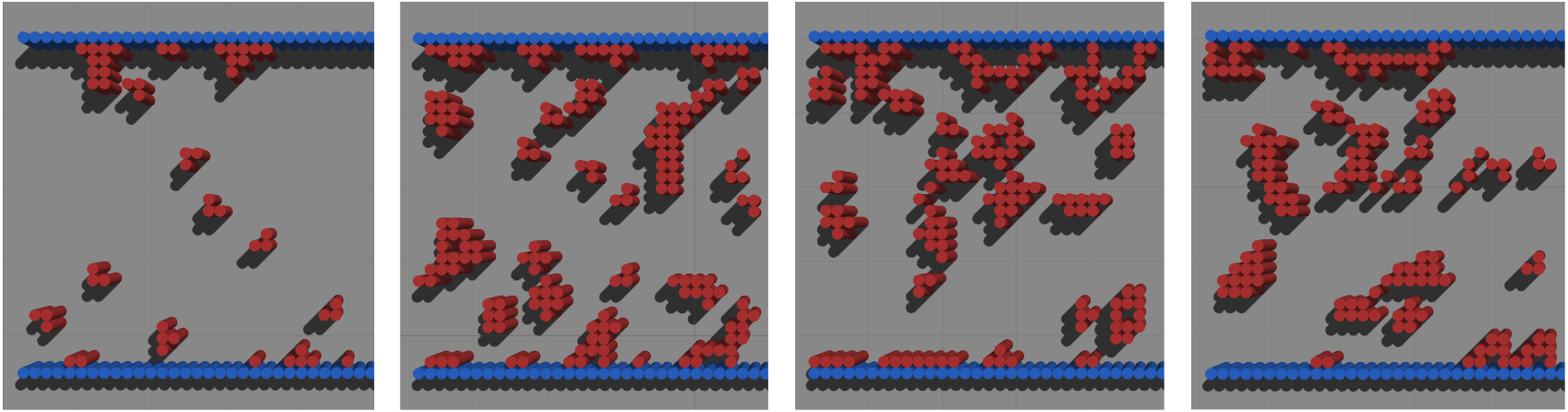
Static environments. We use the 300 static environments from the BARN dataset [20]. The obstacle fields in these environments are represented by a 30$\times$30 black-white grid, which corresponds to an area of 4.5m$\times$4.5m with black and white cells representing obstacle-occupied and free space respectively (see the following figure). The grid cells are generated by a method of cellular automation [21], which is originally designed to generate a collection of black cells on a white grid of specified shape that evolves through a number of discrete time steps according to a set of rules based on the states of neighboring cells. In BARN, such generation process begins with randomly filling the grid cells by a ratio of initial fill percentage, then performs smoothing iterations that either fill an empty cell if the number of its filled neighbors is larger than fill threshold or empty a filled cell if its filled neighbors is smaller than clear threshold. The grids that are not navigable will be discarded. Due to the cellular automation, the resulting grid resembles real-world obstacles more than the initial randomly filled grid does. To generate BARN dataset, 12 different sets of hyper-parameters are used with initial fill percentage chosen from $\{0.15, 0.2, 0.25, 0.3\}$ and smoothing iterations ranges from 2 to 4. The fill threshold and clear threshold are kept at 5 and 1 respectively. Each set of hyper-parameters generates 25 environments which constitute 300 environments in total.
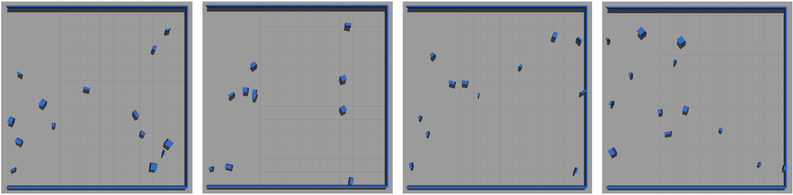
Dynamic box environments. These environments are $13.5m\times13.5m$ obstacle fields (larger than the static environments) that give the agent more time to respond to the moving obstacles (see the following figure). The obstacles are randomly generated without any manually designed challenging scenarios. Each obstacle is a $w\times l \times h$ box with its width $w$ and length $l$ randomly sampled from a range of $[0.1m, 0.5m]$ and a height $h=1m$. The obstacles start from a random position on the left edge of the obstacle field with a random orientation and a constant linear velocity. The magnitude of the velocity is randomly sampled from a range of $[1m/s, 1.5m/s]$, and the direction of the velocity is randomly sampled from all the possible directions pointing into the obstacle field. Each obstacle repeats its motion once it moves out of the obstacle field. Each dynamic box environment has 10 to 15 such randomly generated obstacles.
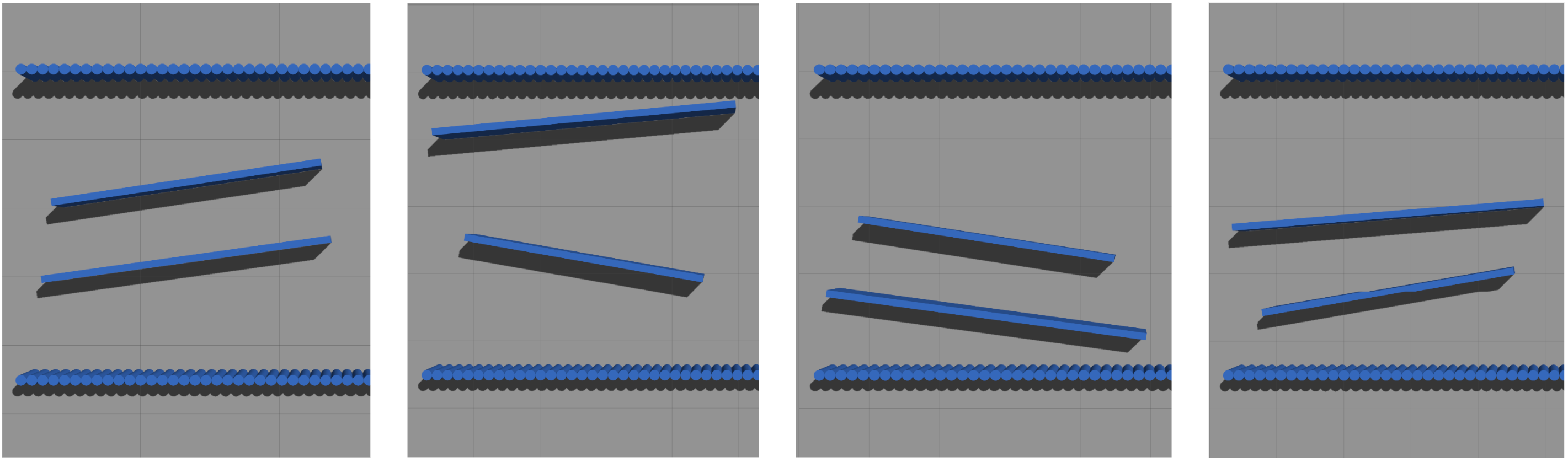
Dynamic wall environments. These environments are $4.5m\times4.5m$, which have two long parallel walls moving in opposite directions with their velocities perpendicular to the start-goal direction (see the following figure). The walls are long enough so that the robot can only pass when the two walls are moving apart. This manually designed navigation scenario requires the agent to maintain a memory of past observations and actions, and to estimate the motion of obstacles. To challenge the agent, we add small variances so that each wall's length, tilting angle, and magnitude of the velocity are randomly sampled from the ranges of $[3.5m, 4.5m]$, $[-10^{\circ}, 10^{\circ}]$ and $[1m/s, 1.4m/s]$ respectively.
Jackal Robot and Navigation system
As shown in the following figure on the left, the navigation is performed by a ClearPath Jackal differential-drive ground robot in navigation environments simulated by the Gazebo simulator. The robot is equipped with a 720-dimensional planar laser scan with a 270$^\circ$ field of view, which is used as our sensory input $\chi_t$. We preprocess the LiDAR scans by capping the maximum range to 5m which covers the entire obstacle field. The goal location $(\bar{x_t}, \bar{y_t})$ is queried directly from the Gazebo simulator. The robot receives velocity commands at a frequency of 5 Hz. A time limit of $80s$ is used which corresponds to a maximum of 400 time steps in an episode. In the real world, the robot is deployed in the same way as simulation except for that the goal location is queried from the on-board ROS move_base stack that localizes the robot simultaneously. The following figure on the right shows a diagram of the RL-based navigation system.

References
[1] R. S. Sutton and A. G. Barto. Reinforcement learning: An introduction. MIT press, 2018.
[2] S. Hochreiter and J. Schmidhuber. Long short-term memory. Neural computation, 9(8):1735–1780, 1997.
[3] J. Chung, C. Gulcehre, K. Cho, and Y. Bengio. Empirical evaluation of gated recurrent neural networks on sequence modeling. arXiv preprint arXiv:1412.3555, 2014.
[4] M. J. Hausknecht and P. Stone. Deep recurrent q-learning for partially observable mdps. In AAAI Fall Symposia, 2015.
[5] D. Wierstra, A. Forster, J. Peters, and J. Schmidhuber. Solving deep memory pomdps with recurrent policy gradients. In ICANN, 2007
[6] A. Vaswani, N. Shazeer, N. Parmar, J. Uszkoreit, L. Jones, A. N. Gomez, L. Kaiser, and I. Polosukhin. Attention is all you need. Advances in neural information processing systems, 30, 2017.
[7] E. Altman. Constrained Markov decision processes: stochastic modeling. Routledge, 1999.
[8] S. Boyd, S. P. Boyd, and L. Vandenberghe. Convex optimization. Cambridge university press, 2004.
[9] C. G. Atkeson and J. C. Santamaria. A comparison of direct and model-based reinforcement learning. In Proceedings of international conference on robotics and automation, volume 4, pages 3557–3564. IEEE, 1997.
[10] G. Thomas, Y. Luo, and T. Ma. Safe reinforcement learning by imagining the near future, 2022.
[11] R. S. Sutton. Integrated architectures for learning, planning, and reacting based on approximating dynamic programming. In Machine learning proceedings 1990, pages 216–224. Elsevier, 1990.
[12] J. A. Rossiter. Model-based predictive control: a practical approach. CRC press, 2017.
[13] J. Tobin, R. Fong, A. Ray, J. Schneider, W. Zaremba, and P. Abbeel. Domain randomization for transferring deep neural networks from simulation to the real world. In 2017 IEEE/RSJ international conference on intelligent robots and systems (IROS), pages 23–30. IEEE, 2017.
[14] F. Sadeghi and S. Levine. CAD2RL: Real single-image flight without a single real image. ArXiv, abs/1611.04201, 2017.448
[15] X. B. Peng, M. Andrychowicz, W. Zaremba, and P. Abbeel. Sim-to-real transfer of robotic control with dynamics randomization. 2018 IEEE International Conference on Robotics and Automation (ICRA), pages 1–8, 2018.
[16] F. Xia, W. B. Shen, C. Li, P. Kasimbeg, M. E. Tchapmi, A. Toshev, R. Martin-Martin, and S. Savarese. Interactive gibson benchmark: A benchmark for interactive navigation in cluttered environments. IEEE Robotics and Automation Letters, 5(2):713–720, 2020.
[17] L. Harries, S. Lee, J. Rzepecki, K. Hofmann, and S. Devlin. Mazeexplorer: A customisable 3d benchmark for assessing generalisation in reinforcement learning. In 2019 IEEE Conference on Games (CoG), pages 1–4. IEEE, 2019.
[18] Y. Zhu, R. Mottaghi, E. Kolve, J. J. Lim, A. Gupta, L. Fei-Fei, and A. Farhadi. Target-driven visual navigation in indoor scenes using deep reinforcement learning. In 2017 IEEE international conference on robotics and automation (ICRA), pages 3357–3364. IEEE, 2017.
[19] E. Marchesini, D. Corsi, and A. Farinelli. Benchmarking safe deep reinforcement learning in aquatic navigation. In 2021 IEEE/RSJ International Conference on Intelligent Robots and Systems (IROS), pages 5590–5595. IEEE, 2021.
[20] D. Perille, A. Truong, X. Xiao, and P. Stone. Benchmarking metric ground navigation. In 2020 IEEE International Symposium on Safety, Security, and Rescue Robotics (SSRR), pages 116–121. IEEE, 2020.
[21] S. Wolfram. Statistical mechanics of cellular automata. Reviews of modern physics, 55(3):601, 1983.
Contact
For questions, please contact:
Dr. Xuesu Xiao
Department of Computer Science
George Mason University
xiao@gmu.edu